Where do you go to my lovely...
… when you are alone in your Slack?
Ever wondered what your colleagues are up to when they are not posting cat videos in #random in your workplace’s Slack? Are they on holidays? Or does their new relationship or project consume most of their time? Find out if and why! Here, in Lucas’ fun-packed world of Slack analysis!
I will demonstrate two rather easy methods for finding behavioral structures in message data exported by Slack, the collaborative messaging software, which literally every hip person/company is using right now. So of course, we (the cool kids) have our private Slack with ca. 60 users. Slack offers the possibility to export all messages sent to public channels. Private messages are private and therefore not accessible. We have taken all the messages from the last 2.5 years and went onto a journey through time.
Note: The names of the users in the data are anonymized.
Slackbot, halt the flow of time!
First, let’s have look at the data at hand. Note that this data set is generated from a sanitized export of slack data. I think, I have ranted enough about data handling in my previous posts, but there you go. From a list of messages, annotated with the user sending it and a timestamp, we aggregated two things. The first one being the number of messages per user per day. The other one tells us about the total number of messages per day for all users. This leaves us with several tables, one for each user and one for the system, which look like this.
| user u005 | |
|---|---|
| timestamp | message_count |
| 2016-08-01 | 200 |
| 2016-08-02 | 42 |
| 2016-08-03 | 99 |
| … | … |
This is called a time series because it maps values to points in time. In our case the message count is mapped to each day for a single user. We will call a user’s timeline user behavior and the complete count of messages system behavior. You might have noticed that I am using the word behavior. This is a very rough approximation of what we understand when we talk about human behavior. Here, we model and therefore simplify a personal behavior to a pattern. In our case the pattern is the history of messages sent to a peer group also known as your social context. The general idea is that we usually behave like our social context. If the activity in such a context rises, we automatically try to follow. Our activity profile tries to level with the system’s degree of activity. Most of the time this does not happen immediately, but with an offset. The user cannot reach an high amount of activity this instant. It takes some time and therefore we can see a small delay between context and user. If we cannot catch up to our social context, there could be a severe personal event blocking us from participating in social activities. This results in some sort of abnormal personal behavior pattern compared to the system behavior. We can apply this to Slack message activity. An active member in a channel will always try to participate in discussions, help others or share videos of children falling over. We are going to quantify this notion in the analysis.
But enough with the conceptual explanations! Here is a graph for user u040 and the system behavior for the complete 2.5 years. The timestamps span from 2015-07-08 to 2018-01-24.
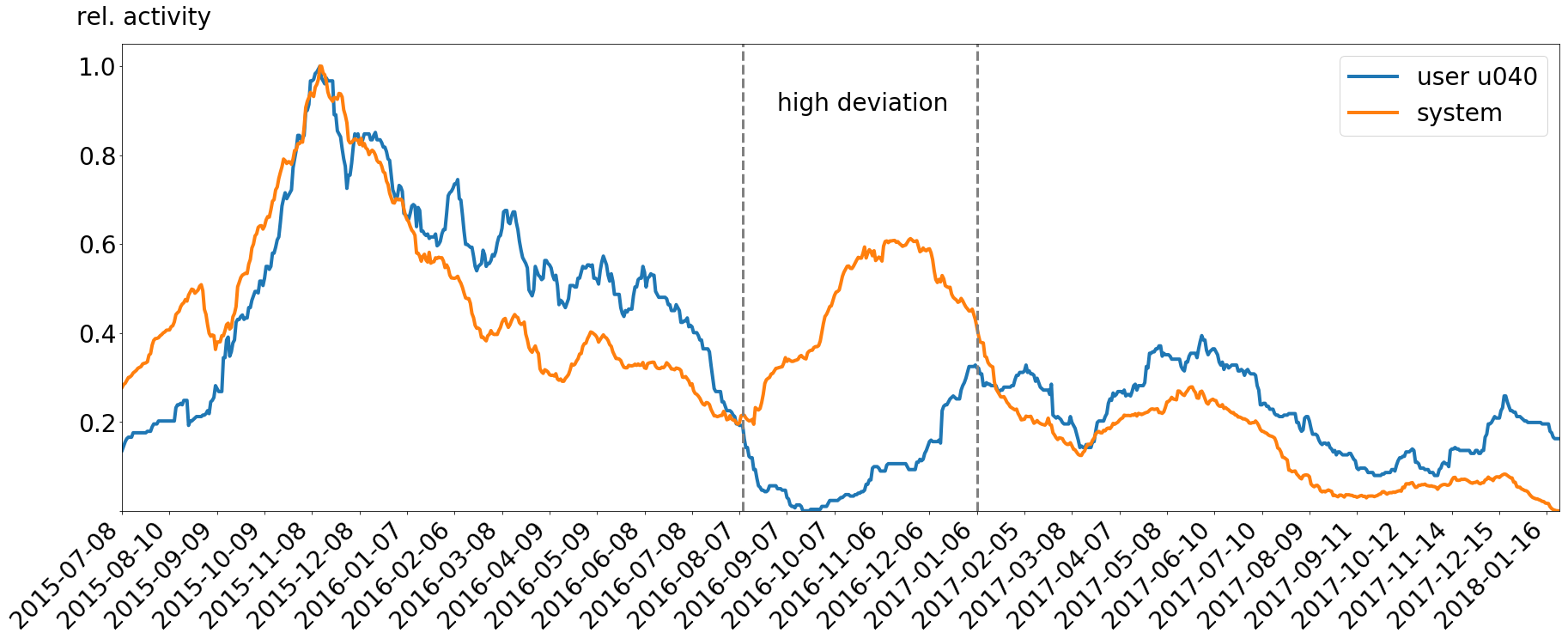
The data is smoothed with a convolution with a factor of 70. Otherwise the curve would be very zigzag, jumping from zero to other values and back again. The y-axis shows the relative activity of messages sent. 1.0 means the maximal amount of messages ever recorded for this user or system, 0.5 means 50% of the maximum of messages and so on. You will notice the seasonality of the data as a first insight. The highs and lows encapsulate semesters as they occur in Germany. The probability for our Slack team to contain student users is very high. Fun fact: it does.
Now, if you take a look at the sample user’s time line and compare it to the system behavior, you will notice the user follows the system with an offset as mentioned in previous paragraphs. As an individual, the user tries to keep up with the current events around him. Nevertheless, there are some points which do not follow our assumption. This range is marked with horizontal lines. Somehow the user does not follow the general behavior of the social context. This is because the user spent this time abroad, removing himself from the usual social context. The user cannot follow the social context as usual. Even though this is visible just by looking at the graph, we will have look into how we can find the approximated start and end point for this event in the next section.
Let’s do the Time Warp again!
No, seriously! The method I will be using throughout this page is called Dynamic Time Warping (DTW). This is pretty cool given the prerequisite that you have watched The Rocky Horror Picture Show. DTW has its application in speech pattern matching and time series forecasting. The technology is used for matching two time series to each other. It maps all points of both series to a common domain (the x-axis) and a common range (the y-values). Imagine having two woolen threads of different length lain out before you in random patterns. By stretching and bending both of them you will be able to make them look the same. The same thing happens to two time series under the influence of DTW. The main concept behind DTW is the shortest path of alteration for the time series to match them. The measure for path optimization are the euclidean distances between the points of both series. I will not go to any more detail, but let me just say that the original algorithm is based on a correction matrix. If we apply DTW to the two time series and mark all found mappings in our graph, we get the following figure.
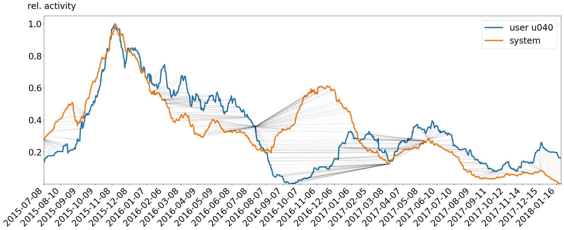
We will use two measures from the mapping. On the one side, we use the distances of the mappings (the black lines) for finding large offsets between the time series and therefore points where the user has a large discrepancy to the social context. The second thing is the number of times a single point gets mapped from one time series to the other to find starts and ends of personal events. These point are indicators for the start or end of an event because the algorithm tries to map extreme derivation between the two timelines to extreme distances. This results in long mapping lines in the graph going to a single point in one of the two time series. These highly mapped nodes occur at the start and the end of the derivation.
Onwards to the first feature! The next figure shows all mapping distances between the two curves. This graph is also smoothed to make the maxima stand out more.
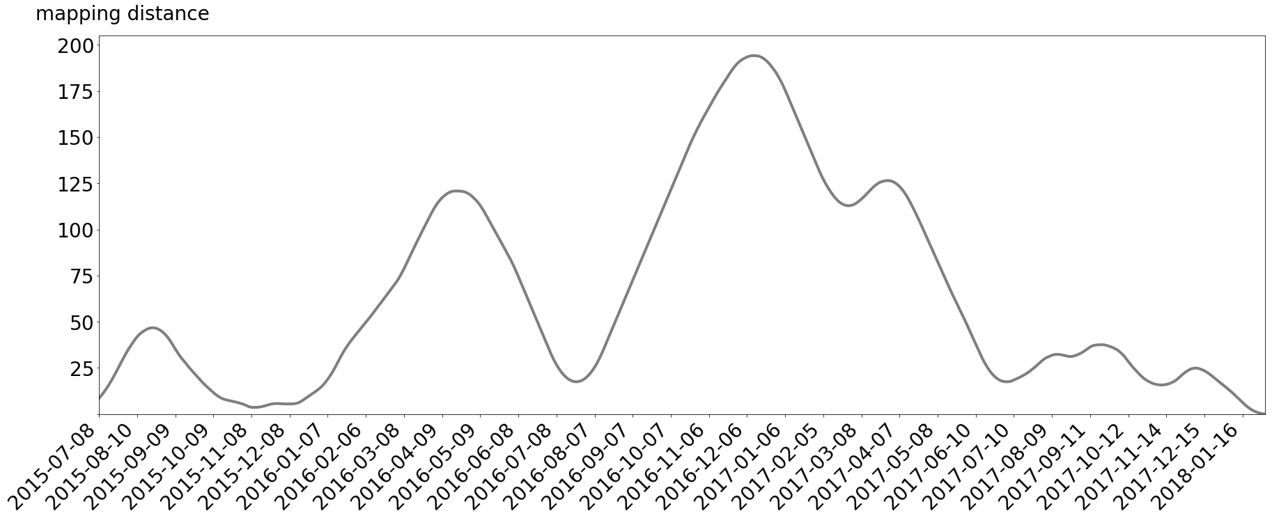
It is immediately visible that the time the user spent abroad (from August 2016 to December 2016) has the longest mapping distances. Still, we do not know the exact dates of leaving and returning.
This can be shown with our second feature, the count of mappings per point. The feature counts how many times each point from the user’s time line is mapped onto the system behavior (black spikes) and how many times the system behavior gets mapped to the user behavior (blue spikes). We have to generate both directions because the algorithm treats the behaviors as equal. We of course know that the user behavior tries to follow the system, so we have to look both ways.
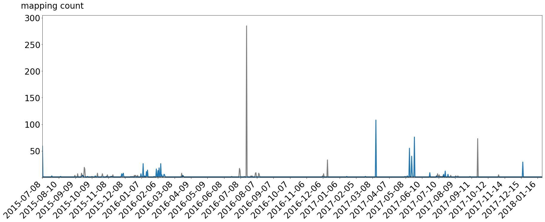
There are three notable spikes in the black user-to-system mapping. These are on 2016-07-19, 2016-12-15 and 2017-09-22. Whereas the first two pretty much show the dates of departure and return with errors of 22 and 7 days respectively, is the third one is another event in the user’s life. And hey, at this point of time the user was in fact moving. Because it is a short event, it only has one spike where there is a lot of mapping. The error for this event is 3 days, making the average error 11 days for all three events.
For the blue system-to-user mapping, we can also see three large peaks. They are on 2017-03-14, 2017-05-24 and 2017-12-18. The last one is the indication for the Christmas holiday season, where users usually do not post many things on Slack. The first spike details the user’s start of his master’s thesis. The last point was just a very busy week for the user, making him write less in Slack. The errors for these events are 4 days, 0 days, 5 days and therefore 3 days on average.
You can see, we might not get all events of a user, but we certainly find a lot of interesting points in a user’s life. We will now go further and analyze behavior changes between two users.
Wi nøt trei a høliday in Sweden this yër?
We have analyzed the deviation of a single user, but this is not the end of the flag pole. If we can manage to expand our insights to two or more users, we can find special relationship events between them. First of all, let me show you an additional user to our previous one.
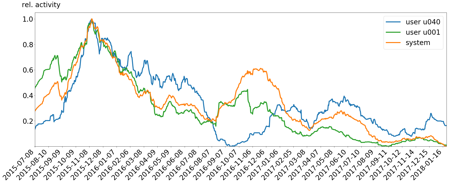
The user u001 follows the system much closer compared to user u040. If we do the same thing, we did for user u040, for user u001, we can compare their mapping distances in one graph.
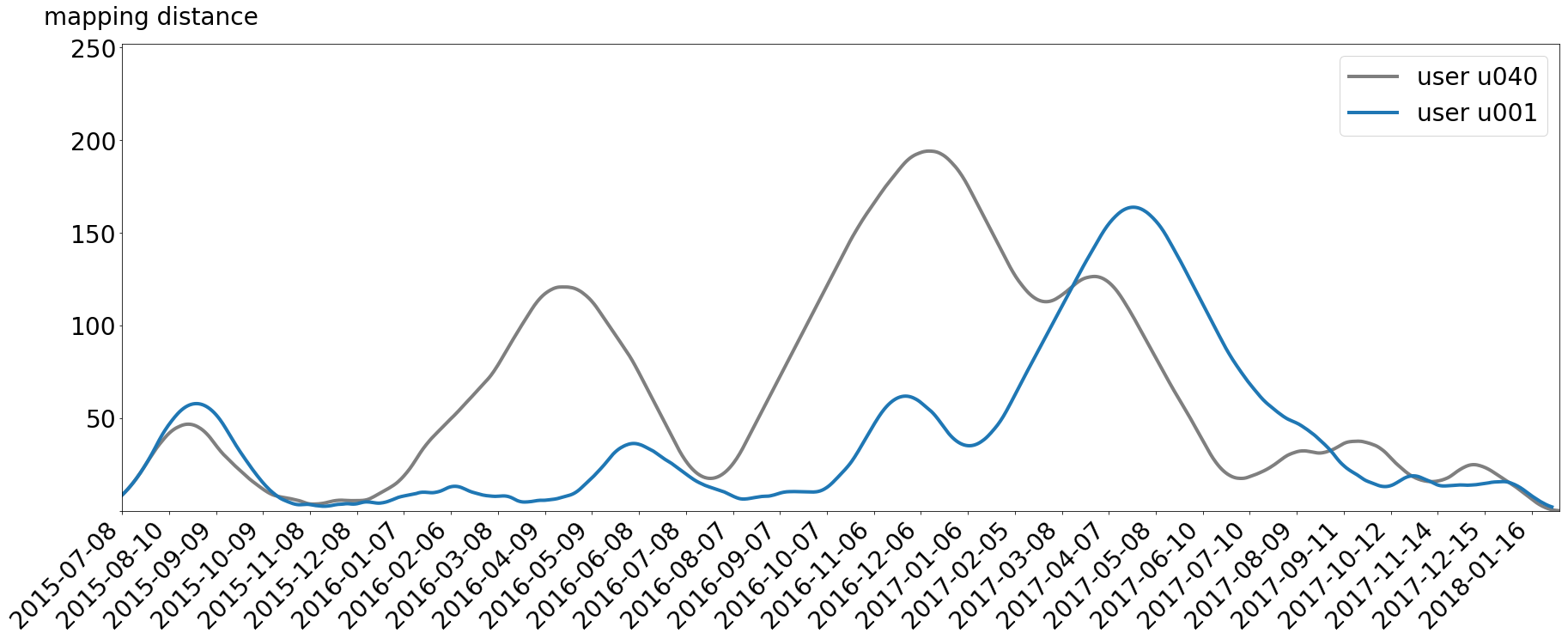
The good thing is, we now can see where the users experience the same amount of deviation from the system based on their mapping to the system. If the distance curves behave the same, there could be an event which was important to both users. High distances occurring simultaneously mean that both users diverted from the system at the same time with the same relative amount of activity lost. In our case there is one nearly identical part of peaks around 2015-09-27 and 2015-09-18. And you would not dreamed about it but this is the time the two users spent their holidays together. They both retreated from their social context, but they did it nearly in the same way. So, our analysis can show this correlation. This can be expanded to other alignments, like joint projects and relationships.
Working hard or hardly working?
We have seen that it is pretty simple to generate insights from activity protocols. Of course, our approach gives neither all important events of a user nor does it provide any information about what happened. The only thing it can tell you is whether an influential event occurred. The astonishing thing is how close we can model a user with so little data. This is due to the high integration of Slack into our everyday life. We share a lot of things in this environment even if we are not actively aware of it. Imagine the possibilities if you had an even better view on a user’s day-to-day activities or a better analyst.
I admit that the evaluation of the algorithm is not very sound. The problem here is that I would have to go to everybody with all my analyses and say stuff like, “What did you do on 2017-09-01? Was there anything special in that particular week?” This seems nosy and annoying to most people. I have checked with several other people, but I cannot show you everything because of the focus of this post and privacy concerns. I am currently thinking about a good way to measure the prediction with precision and recall.
Another major problem is the different inertia of users. Even if the system starts a time period with high activity some users need up to 7 days before getting to the level of the system. The problem is not that there is no rise in activity for those users, but the slope of the activity curve is much flatter than the system’s slope. This is because the system aggregates all user activity and therefore has a steeper slope for changes in activity. “Slow” users have a higher derivation than people with “fast” reactions in these areas. This makes the mapping sloppy and our algorithm produces events for these slow-pace users where there might be none.
Still, there is a lot of potential here. One could analyze the sentiment of each text message and correlate the mood of a user to the count of the messages per day. This would give more information about an event being positive or negative instead of just the knowledge of an event happening. Jolly language can indicate a pleasant event in the user’s life, a rude or even aggressive tone could show that the user has a bad day. A similar approach would be to examine the gradient of the user behavior at found events to model retreating from or reentering to the social context. A steep fall in activity could be seen as a event resulting in withdrawal from the social context.
I hope you see how very interesting this topic is and how much research potential it bears. And therefore back to our Slack admins, bearer of great no responsibility.
Other sources and libraries include pandas, numpy, matplotlib, jupyter and of course Slack.